Hashing Collision Resolution - Double Hashing Formula & Example
<<Previous - Quadratic Probing
Double Hashing algorithm
Double hashing is a computer programming technique. Double hashing is hashing collision resolution technique
Double Hashing uses 2 hash functions and hence called double hashing.
Before understanding double hashing. Let us understand What is hashing?
What is hashing?
Hashing is the process of simplifying a lengthy value into a small value called the hash. Let us say 10 words are converted into its hash. Most times, there would be 10 hash one each for one word. However, sometimes, few values may end up having the same hash value. This clash of same hash value for multiple words is called a collision.
To resolve the collision, we can use double hashing
- Hashing technique uses 1 hash function.
- Double Hashing uses 2 hash functions.
Double Hashing and Open Addressing help to create the popular data structure called Hashtable or Hashmap. Open addressing is another collission resolution technique just like double hashing
Double Hashing - Hash Function 1 or First Hash Function - formula
where
- F(i) = i * hash2(X)
- X is the Key or the Number for which the hashing is done
- i is the ith time that hashing is done for the same value. Hashing is repeated only when collision occurs
- Table size is the size of the table in which hashing is done
This F(i) will generate the sequence such as hash2(X), 2 * hash2(X) and so on.
Double Hashing - Hash Function 2 or Second Hash Function - formula
Second hash function is used to resolve collission in hashing
We use second hash function as
where
- R is the prime number which is slightly smaller than the Table Size.
- X is the Key or the Number for which the hashing is done
Double Hashing Example - Closed Hash Table
Let us consider the same example in which we choose R = 7.
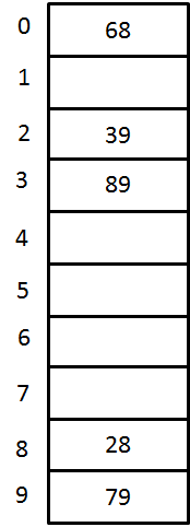
A Closed Hash Table using Double Hashing
Key Hash Function h(X) Index Collision Alt Index 79 h0(79) = ( Hash(79) + F(0)) % 10
= ((79 % 10) + 0) % 10 = 99 28 h0(28) = ( Hash(28) + F(0)) % 10
= ((28 % 10) + 0) % 10 = 88 39 h0(39) = ( Hash(39) + F(0)) % 10
= ((39 % 10) + 0) % 10 = 99 first
collision
occursh1(39) = ( Hash(39) + F(1)) % 10
= ((39 % 10) + 1(7-(39 % 7))) % 10
= (9 + 3) % 10 =12 % 10 = 22 2 68 h0(68) = ( Hash(68) + F(0)) % 10
= ((68 % 10) + 0) % 10 = 88 collision
occursh1(68) = ( Hash(68) + F(1)) % 10
= ((68 % 10) + 1(7-(68 % 7))) % 10
= (8 + 2) % 10 =10 % 10 =00 0 89 h0(89) = ( Hash(89) + F(0)) % 10
= ((89 % 10) + 0) % 10 = 99 collision
occursh1(89) = ( Hash(89) + F(1)) % 10
= ((89 % 10) + 1(7-(89 % 7))) % 10 = (9 + 2) % 10 =10 % 10 = 00 Again
collision
occursh2(89) = ( Hash(89) + F(2)) % 10
= ((89 % 10) + 2(7-(89 % 7))) % 10 = (9 + 4) % 10=13 % 10 =33 3
<<Previous - Quadratic Probing